General Topology

Syllabus 2021 and Class board – any public or private questions are welcome.

Contents

Introduction
Basic concepts
Selected topics
Interesting reading articles
Homework #1
Homework #2
Homework #3
Homework #4
Homework #5

Brief Introduction

Geometry and Topology provide distinct perspectives of the same thing. On the one hand, Geometry provides a quantitative perspective on spaces, i.e., we measure lengths, areas, volumes, or curvatures, etc. to study spaces. On the other hand, Topology provides a qualitative perspective on spaces, i.e., we study the properties of spaces that are invariant under continuous deformation such as connectivity, continuity, etc.

In the field of Topology, there are subfields such as general topology, differential topology, algebraic topology. General topology is the most fundamental, which we cover in this course. Differential topology and algebraic topology use differential and algebraic structures in the study of spaces as the names indicate. There is also surface topology that characterizes all 2 dimensional (orientable or non-orientable) manifolds.

Interestingly, Topology turns out to play a crucial role in data analysis. For example, when we collect data points in a high dimensional space, we would like to determine the connectivity among the points, which is a typical question related to Topology. Indeed, there are quite a few works on the link between topology and data analysis. To name a few, we have the following references:

G. Carlsson, Topology and data, Bull. AMS, Vol. 46, No. 2, pp.255–308, 2009
H. Edelsbrunner and J. Harer, Persistent homology: A survey, Surveys on Discrete and Computational Geometry. Twenty Years Later, Contemporary Mathematics, Vol 453, AMS, 2008
F. Chazal and B. Michel, An introduction to Topological Data Analysis: fundamental and practical aspects for data scientists, arXiv:1710.04019v2, 2021

In this course, we begin discussing the basics of Topology. It is always good to have concrete examples for better understanding of abstract notions, for which students need to work out problems. Towards the end of the semester, I will try to present briefly how topology applies to data science through examples.

Basic Concepts

Definition 1) A topology on a set $X$ is a collection $\mathcal{J}$ of subsets of $X$ having the following properties:

$\emptyset$ and $X$ are in $\mathcal{J}$ .
The union of the elements of any subcollection of $\mathcal{J}$ is in $\mathcal{J}$ .
The intersection of the elements of any finite subcollection of $\mathcal{J}$ is in $\mathcal{J}$ .

A set $X$ for which a topology $\mathcal{J}$ has been specified is called a topological space.

Below is an example of a topology: the collection of all open subsets of $\mathbb{R}$ is a topology on $\mathbb{R}$ according to Definition 1) above.

Example BC1) Knowing that $\mathbb{R}$ is a metric space with the standard metric $d(a,b) = |a-b|$ , we say that a subset $U\subset \mathbb{R}$ is open if $\forall x\in U$ , there exists $r>0$ such that $(x-r,x+r)\subset U.$

Let $\mathcal{J}$ be the collection of all open subsets of $\mathbb{R}$ . We can see that $\mathcal{J}$ is a topology on $\mathbb{R}$ as follows.

1) Remembering that $U$ is open if and only if $U^c$ is closed, we can see that $\emptyset$ and $X$ are both open.

2) Let $\{U_k\}_{k\in K}$ be a collection of open subsets $U_k$ in $\mathbb{R}$ . Since the number of elements in $\{U_k\}_{k\in K}$ is $K$ , which can be either finite or infinite (countable or uncountable), $\{U_k\}_{k\in K}$ can be any subcollection of $\mathcal{J}$ . We can see that $\cup_{k\in K} U_k$ is an open subset of $\mathbb{R}$ , i.e., $\bigcup_{k\in K}U_k\in \mathcal{J}.$

To see this, we choose an arbitrary element $x\in \cup_{k\in K}U_k$ . Since there exists $l\in K$ such that $x\in U_l$ and $U_l$ is open, there exists $r>0$ such that $(x-r,x+r)\subset U_l$ . That is, $(x-r,x+r)\in \cup_{k\in K}U_k$ . This implies that $x$ is an interior point of $\cup_{k\in K}U_K$ . So, any element in $\cup_{k\in K}U_k$ is an interior point. Hence, $\cup_{k\in K}U_k$ is open.

3) Let $\{U_k\}_{k\in K}$ be a finite collection of open subsets $U_k$ in $\mathbb{R}$ . We may consider $\{U_1,\dots, U_K\}$ for some $K\in\mathbb{N}$ . To see that $\cap_{k=1}^KU_k$ is open, we choose any $x\in\cap_{k=1}^KU_k$ and show that $x$ is an interior point. In fact, for $x\in\cap_{k=1}^KU_k$ , there exists $r_1,\dots, r_K>0$ such that

$(x-r_k, x+r_k)\subset U_k,\quad k=1,2,\dots, K.$

Let $r:=\min(r_1,\dots,r_K)$ . Then, it is obvious to see that $(x-r,x+r)\subset U_k$ for all $k=1,2,\dots,K$ . That is, $(x-r,x+r)\subset \cap_{k=1}^KU_k$ . Hence, $x$ is an interior point of $\cap_{k=1}^KU_k$ . This means that $\cap_{k=1}^KU_k$ is an open subset of $\mathbb{R}$ , i.e., $\bigcap_{k\in K}U_k \in \mathcal{J}.$

The same is true for $\mathbb{R}^n$ for any $n\in\mathbb{N}$ : the collection of all open subsets of $\mathbb{R}^n$ is a topology on $\mathbb{R}^n$ . Therefore, the concept of a topology on $X$ generalizes that of open sets in $\mathbb{R}^n$ . In other words, a topology on any set $X$ decides which subsets of $X$ are considered open in $X$ .

Homework #1 – Due on 9/21 Tuesday.

Problem#1) Let $(X,\mathcal{T})$ be a topological space. Let $S\subset X$ . Let $\mathcal{T}_S = \{ U\cap S : U \in \mathcal{T}\}$ . Prove that $\mathcal{T}_S$ is a topology on $S$ .

Problem#2) Let $X$ be a topological space. Let $S\subset X$ .
a) If $S$ is open in $X$ , then prove that $S\subset \text{int}(\overline{S})$ .
b) If $S$ is closed in $X$ , then prove that $\overline{\text{int}(S)}\subset S$ .

Problem#3) Let $\mathbb{R}$ be the one-dimensional Euclidean space with the Euclidean metric. Let $X = \mathbb{R}\cup\{\infty\}$ . Let $\mathcal{T}$ be a collection of subsets of $X$ such that $\emptyset, X\in\mathcal{T}$ and
i) $U\in \mathcal{T}$ for any open set $U$ in $\mathbb{R}$ ,
ii) $U\cup\{\infty\}\in \mathcal{T}$ for any open set $U$ in $\mathbb{R}$ satisfying $(-\infty, a)\cup(b,\infty)\subset U$ for some $a<b$ .
a) Prove that $\mathcal{T}$ is a topology on $X$ .
b) Prove that $X$ is topologically equivalent to the unit circle.

Problem#4) Section 2.1: #1, #3, #7, #8

Problem#5) Section 2.2: #1, #2, #4

Homework #2 – Due on 10/11 Monday.

Problem#1) Let $A$ be a collection of subsets of a topological space $X$ such that $\emptyset, X\in A$ . Let $\mathcal{T}_A$ be the smallest topology containing $A$ . We say that $A$ is a subbase for the topology on $X$ . We now consider a collection $\mathcal{B}$ of all finite intersections of elements of $A$ . Prove that $\mathcal{B}$ is a base for the topology on $X$ .

Problem#2) We consider a product space $X\times Y$ given two topological spaces $X, Y$ . Let $\pi_1:X\times Y\to X$ and $\pi_2:X\times Y\to Y$ be projections defined by $\pi_1(x,y) = x$ and $\pi_2(x,y) = y$ for all $x\in X,\ y\in Y$ . Prove that
$A = \{\pi_1^{-1}(U) : U\text{ is open in }X\}\cup\{\pi_2^{-1}(V) : V\text{ is open in }Y\}$ is a subbase for the product topology on $X\times Y$ .

Problem#3) A topological space $X$ is first-countable if for each $x\in X$ , there exists a sequence of open neighborhoods $\{U_n\}_{n=1}^\infty$ of $x$ such that each neighborhood of $x$ includes one of the $U_n$ ‘s.
i) Let $X$ be first-countable. Let $S\subset X$ . Prove that any point adherent to $S$ is a limit of a sequence in $S$ .
ii) Let $X=\mathbb{R}$ have the topology $\mathcal{T}$ given in Example 3.1 in the lecture note. Prove that $(X,\mathcal{T})$ is not first-countable.

Problem#4) Section 2.3: #9, #12

Problem#5) Section 2.4: #6(c)(d), #8(b)(c)(d)

Homework #3 – Due on 11/14 Sunday.

Problem#1) Prove that connectedness defines an equivalence relation. In other words, if we we define $\sim$ by $x\sim y$ if and only if $C(x) = C(y)$ , where $C(x)$ is the connected component in a topological space $X$ containing $x\in X$ , then $\sim$ is an equivalence relation on $X$ .

Problem#2) Prove that a topological space $X$ is normal if and only if the conclusion of Urysohn’s lemma is valid for $X$ .

Problem#3) Section 2.5: #1, #9(a)(b)(c)(d)(e)

Problem#4) Section 2.6: #2, #6, #7, #8, #10, #11

Homework #4 – Due on 11/28 Sunday.

Problem#1) Section 2.7: #1, #3

Problem#2) Section 2.8: #6, #7, #9, #10, #11, #14

Problem#3) Section 2.9: #4, #7

Problem#4) Section 2.10: #1, #2

Homework #5 – Due on 12/12 Sunday.

Problem#1) Section 2.13: #1(a)(b)(c), #4, #6, #8(a)(c)(d), #9(a)(b)

Problem#2) Find a homeomorphism $f:S^1\times S^1\to\mathbb{T}$ , where $\mathbb{T}$ is the torus.

Problem#3) Complete the proof that the homotopy equivalence is an equivalence relation on the collection of topological spaces. That is to prove that the relation $\sim$ on the collection of topological spaces is an equivalence relation, defined as follows: two topological spaces $X, Y$ being homotopic equivalent if and only if there exists a homotopy equivalence $f:X\to Y$ .

Problem#4) A topological space $X$ is said to be simply-connected if it is path-connected and the fundamental group $\pi_1(X,x_0) = \{0\}$ . Prove that the following three are equivalent:
1. Every map $S^1\to X$ is homotopic to a constant map,
2. Every map $S^1\to X$ extends to a map $D^2\to X$,
3. $\pi_1(X,x_0) = \{0\}$ for all $x_0\in X$ .

Selected Topics

Various types of topologies

Let $X$ be a set. Let $\mathcal{T}$ be a topology on $X$ . Then, we may consider continuous functions on $X$ . Please remember that the continuity of a function $f$ depends on the topology $\mathcal{T}$ .

Let $\mathcal{T}_1$ be another topology on $X$ that is finer than $\mathcal{T}$ , i.e., $\mathcal{T}\subset \mathcal{T}_1$ . It is easy to see that a function $f:X\to\mathbb{R}$ is continuous with respect to $\mathcal{T}_1$ if it is continuous with respect to $\mathcal{T}$ . This implies that if we find the smallest topology $\mathcal{T}$ for which a given function $f:X\to\mathbb{R}$ is continuous, then $f$ is continuous with respect to any other topologies containing $\mathcal{T}$ (or finer than $\mathcal{T}$ ). In the same way, considering a set of functions

$A=\{ f_i:X\to\mathbb{R} : i\in I\}$ ,

we may consider the smallest topology $\mathcal{T}$ for which all the functions in the set $A$ are continuous.

Exercise ST1) Let $f_i:\mathbb{R}\to\mathbb{R}$ be defined by $f_i(x) = 1_{[i,i+1)}(x)$ for $i\in\mathbb{Z}$ .
1. The smallest topology $\mathcal{T}_i$ on $\mathbb{R}$ for which $f_i$ is continuous is $\mathcal{T}_i = \{\emptyset, [i,i+1), \mathbb{R}, (-\infty,i)\cup[i+1,\infty)\}$ .
2. The smallest topology $\mathcal{T}$ on $\mathbb{R}$ for which all $f_i$ ‘s are continuous is generated by $\{[i,i+1) : i\in\mathbb{Z}\}$ , i.e., $\mathcal{T}$ consists of arbitrary unions of the half-open intervals in $\{[i,i+1) : i\in\mathbb{Z}\}$ together with $\emptyset, \mathbb{R}\in\mathcal{T}$ .

Exercise ST2) Let $V$ be an $n$ -dimensional real vector space. Then, $V$ is naturally endowed with the Euclidean topology of $\mathbb{R}^n$ .
1. Let $\beta=\{\mathbf{v}_1,\dots,\mathbf{v}_n\}$ be a basis for $V$ . Let $\tilde{\beta}=\{\mathbf{e}_1,\dots,\mathbf{e}_n\}$ be the standard basis for $\mathbb{R}^n$ . Then, we can see that the natural topology on $V$ is $\{ f^{-1}(B) : B\ \text{ is open in }\ \mathbb{R}^n\}$ , where $f:V\to \mathbb{R}^n$ is defined by $f\left(\sum_{i=1}^n a_i\mathbf{v}_i\right) = \sum_{i=1}^n a_i\mathbf{e}_i$ . With the natural topology on $V$ , we note that $f:V\to\mathbb{R}^n$ is continuous.
2. In linear algebra, there is an important concept of a dual space $V^*$ to the vector space $V$ . The dual space $V^*$ is the set of all linear functionals on $V$ . A linear functional $f$ on $V$ is a linear function from $V$ to $\mathbb{R}$ . In fact, the dual space is an $n$ -dimensional real vector space with a basis $\{\mathbf{v}_1^*,\dots,\mathbf{v}_n^*\}$ such that $\mathbf{v}_j^*(\mathbf{v}_l) = \delta_{jl}$ . That is, we have
$V^*=\left\{\sum_{i=1}^n a_i\mathbf{v}_i^* : a_i\in\mathbb{R}\right\}$ . Noting that each element $\sum_{i=1}^n a_i\mathbf{v}_i^*$ in $V^*$ is a linear function from $V$ to $\mathbb{R}$ , we may consider the smallest topology on $V$ such that all the elements in $V^*$ are continuous. Is this smallest topology the same as the natural topology that we discussed above or different? This smallest topology is called the weak topology on $V$ .

Exercise ST3) As we have seen in Exercise SP2, we may define the weak topology on the vector space $V^*$ . In other words, the weak topology on $V^*$ is the smallest topology on $V^*$ for which all linear functionals on $V^*$ are continuous. Note that the set of all linear functionals on $V^*$ is the dual space of $V^*$ denoted by $V^{**}=(V^*)^*$ . It is interesting to observe that each element $\mathbf{v}\in V$ can be identified with a linear functional $f$ on $V^*$ defined by $f_\mathbf{v}(a\mathbf{v}_1^* + b\mathbf{v}_2^*) := a\mathbf{v}_1^*(\mathbf{v}) + b\mathbf{v}_2^*(\mathbf{v})$ for $a\in\mathbb{R}$ and $\mathbf{v}_1^*,\mathbf{v}_2^*\in V^*$ . It is through this identification $\mathbf{v} = f_\mathbf{v}$ that we end up with $V\subset V^{**}$ . Beside the weak topology on $V^*$ that makes all the elements in $V^{**}$ continuous, we may define another topology on $V^*$ called the weak- $*$ topology (say weak-star) on $V^*$ for which all the elements in $V$ identified as elements in $V^{**}$ are continuous. It is interesting to see that $V=V^{**}$ when $V$ is of finite dimensional. However, for an infinite dimensional vector space $V$ , we have $V\subsetneq V^{**}$ , in general.

More will be discussed in class about the weak and the weak- $*$ topologies.

Manifolds Triangulation

For simplicity, we consider an $n$ -dimensional topological manifold, which is a topological space $M$ with a property that it looks locally like the $n$ -dimensional Euclidean space. By the local resemblance to the $n$ -dimensional Euclidean space, we mean that for any $p\in M$ , there exists a homeomorphism $\phi: U\to V$ , where $U$ is an open neighborhood of a point $p\in M$ and $V$ is an open neighborhood of $\phi(p)\in\mathbb{R}^n$ . A topological manifold is a differentiable manifolds when the homeomorphisms are replaced by diffeomorphisms. In this lecture, we will only consider topological manifolds. Hence, a topological manifold is simply referred to as a manifold.

Exercise ST4) Let $M = S^n$ , the $n$ -dimensional sphere defined by

$S^n = \{(x_1,\dots,x_{n+1})\in\mathbb{R}^{n+1} : x_1^2+\cdots + x_{n+1}^2 = 1\}.$

1. Define a topology on $M$ to make it an $n$ -dimensional topological manifold.
2. Under the chosen topology, write down a homeomorphism $\phi$ from an open neighborhood of $(0,0,\dots,0,1)$ to an open neighborhood of $\phi(0,0,\dots,0,1)$ .

A triangulation on an $n$ -dimensional manifold is a representation of the manifold in terms of $n$ -simplexes.

Definition 1) An $n$ –simplex is a convex hull of $n+1$ vertices in $n$ -dimensional space that do not lie simultaneously in any $n-1$ -dimensional subspace:

Example 1) A $0$ –simplex is a point. A $1$ -simplex is a line segment. A $2$ -simplex is a triangle. A $3$ -simplex is a tetrahedron, etc. To view an $n$ -simplex, you may consider an $n$ -dimensional Euclidean space and take the $(n+1)$ number of points $p_0,p_1,\dots,p_{n}$ chosen by

$p_j = (0,0,\dots,0, 1, 0,\dots, 0),\ j=1,2,\dots,n$

where the only nonzero component in $p_j$ is at the $j^{th}$ component for $j=1,2,\dots,n$ and $p_0$ is the origin. The smallest convex set containing all the points $p_0,p_1,\dots,p_n$ is an $n$ -simplex. It is interesting to see that every face of this $n$ -simplex consists of $n$ points $\{p_0,p_1,\dots,p_n\}\setminus\{p_j\}$ , which constitute an $(n-1)$ -simplex.

It will be easier to see this with a tetrahedron, a $3$ -simplex, having four vertices $p_0=(0,0,0), p_1=(1,0,0), p_2 = (0,1,0), p_3=(0,0,1)$ . If we choose $p_0,p_2,p_3$ , then these three points constitute one face of the tetrahedron, a $2$ -simplex, which is a triangle. If we further choose $p_2,p_3$ from the $2$ -simplex, then these constitute one side of a triangle, a $1$ -simplex, which is a line segment. See below.

Definition 2) A simplicial complex is an object that one can construct by gluing simplexes together along the faces.

Question 1) Does a manifold admit a triangulation? In other words, is it possible to represent an $n$ -dimensional topological manifold by gluing together $n$ -simplexes?

Partial answer 1) Every smooth manifold admits a triangulation, which can be confirmed by the following two papers:

1. Stewart S. Cairns, Triangulation of the manifold of class one, Bull. Amer. Math. Soc. 41 (1935), no. 8, 549–552.
2. John Henry C. Whitehead, On $C^1$ -complexes, Ann. of Math. (2) 41 (1940), 809–824.

Delaunay Triangulation

I, myself, have written a simple MATLAB code below to generate uniform points on a sphere $S^2$ with a prescribed minimum distance between any two points and to visualize the delaunay triangulation:

%
%   Delaunay Triangulation on a sphere
%
clear;close all;

min_dist = 0.2;     % minimum distance between any two points 

xy_pts = 60 ;       % number of equidistanced points on [0, 2*pi)
z_pts  = 20 ;       % number of equidistanced points on (0, pi)

%% Take uniform sample points on the \theta-\phi plane:  0 <= \theat < 2pi, 0< \phi < pi

cnt = 0;
for j1=1:xy_pts
    a = 2*pi*(j1-1)/xy_pts;
    for j2=1:z_pts
        b = pi*j2/(z_pts+1);
        cnt = cnt +1;
        X(cnt,1:3) = [sin(b)*cos(a) sin(b)*sin(a) cos(b)];
    end
end

X = [0,0,1;X;0,0,-1];   % The north and the south poles are added.

%% We remove points within the specified minimum distance.

for j1=1:cnt+2
    for j2=1:cnt+2
        if j2~=j1 && norm(X(j1,:)-X(j2,:))< min_dist && norm(X(j1,:))>0
            X(j2,:) = [0,0,0];
        end
    end
end

cnt1=0;
for j1=1:cnt+2
    if norm(X(j1,:))>0
        cnt1=cnt1+1;
        Y(cnt1,1:3) = X(j1,:);
    end
end

%% Visualization of the delaunay triangulation

Number_Of_Pts = cnt1;   % The total number of points on a sphere

T = delaunayn(Y);

%% Below is to color the tetrahedra.
nT = size(T,1);
C = zeros([nT,1]);  % Colormap
for j1=1:nT
    j1
    C(j1) = 1+floor(10*Y(T(j1,1),3));
end
tetramesh(T,Y,C);

set(gca,'Position',[0.03 0.03 0.95 0.95]);
set(gcf,'Position',[200 200 700 700]);

This code generates the following triangulation.

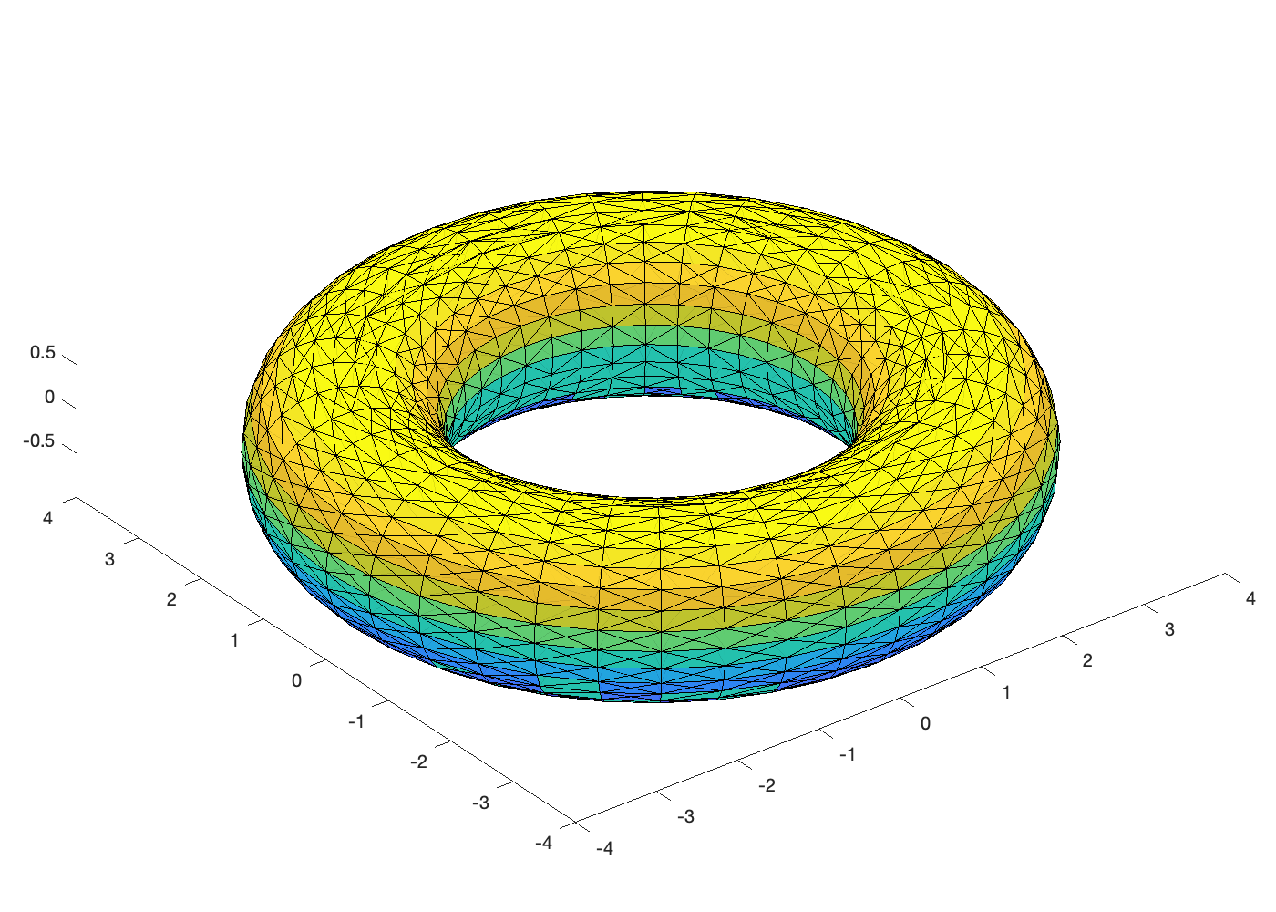
I, myself, have written another simple MATLAB code to generate uniform points on a torus $T^2$ with a prescribed minimum distance between any two points and to visualize the delaunay triangulation. (While I did not do it, the barycenters of tetrahedrons should be compared to remove unwanted connections between points in the code.)

%
%   Delaunay Triangulation on a torus
%
clear;close all;

min_dist = 0.2;     % minimum distance between any two points 

xy_pts = 60 ;       % number of equidistanced points on [0, 2*pi)
z_pts  = 40 ;       % number of equidistanced points on (0, 2*pi)

%% Take uniform sample points on the \theta-\phi plane:  0 <= \theat < 2pi, 0< \phi < 2*pi

cnt = 0;
for j1=1:xy_pts
    a = 2*pi*(j1-1)/xy_pts;
    for j2=1:z_pts
        b = 2*pi*(j2-1)/z_pts;
        cnt = cnt +1;
        X(cnt,1:3) = [-(3+cos(a))*sin(b) (3+cos(a))*cos(b) sin(a)];
    end
end

%% We remove points within the specified minimum distance.

for j1=1:cnt
    for j2=1:cnt
        if j2~=j1 && norm(X(j1,:)-X(j2,:))< min_dist && norm(X(j1,:))>0
            X(j2,:) = [0,0,0];
        end
    end
end

cnt1=0;
for j1=1:cnt
    if norm(X(j1,:))>0
        cnt1=cnt1+1;
        Y(cnt1,1:3) = X(j1,:);
    end
end

%% Visualization of the delaunay triangulation

Number_Of_Pts = cnt1;   % The total number of points on a sphere

DT = delaunayTriangulation(Y);
Num_DT = size(DT,1);

% Below is to remove unwanted connections between points due to the
% nonconvex shape of the torus
cnt2=0;
for j1=1:Num_DT
    coords = DT.ConnectivityList(j1,:);
    z = Y(coords(1),:) + Y(coords(2),:) + Y(coords(3),:) + Y(coords(4),:);
    z = z/4;
    b = 3*z(1:2)/norm(z(1:2));
    b = [b,0];
    if norm(z-b)<=1
        cnt2 = cnt2+1;
        TRI0(cnt2,:) = coords;
    end
end
TR = triangulation(TRI0, Y(:,1),Y(:,2),Y(:,3));

%% Below is to color the tetrahedra

nT = size(TR,1);
C = zeros([nT,1]);  % Colormap
for j1=1:nT
    max_TR = max(Y(TR(j1,1),3),Y(TR(j1,2),3));
    max_TR = max(max_TR,Y(TR(j1,3),3));
    max_TR = max(max_TR,Y(TR(j1,4),3));
    C(j1) = 1+floor(10*max_TR);
end
%%
tetramesh(TR,C);

set(gca,'Position',[0.06 0.04 0.9 0.94]);
set(gcf,'Position',[200 200 700 500]);

This code generates the following triangulation.

Exercise ST5) Write your own MATLAB code to generate a delaunay triangulation on the following C shape. Since you can get the shape by cutting the above torus in half and cap the two ends by the half spheres, you can combine the above two codes if you like.

Euler Characteristic

Definition 1) Let $P$ be a polyhedron with $V$ vertices, $E$ edges, and $F$ faces. The Euler characteristic of $P$ , denoted by, $\chi(P) = V-E+F$ .

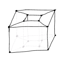
Example EC1) We can consider the following polyhedra.

For a regular cube $C$ in 3D, $\chi(C) = 8 - 12 + 6 = 2$ .
For a regular tetrahedron $T$ in 3D, $\chi(T) = 4 - 6 + 4 = 2$ .
For a regular icosahedron $I$ in 3D, $\chi(I) = 12 - 30 + 20 = 2$ .

It is interesting to observe that the above mentioned polyhedra can be drawn on the surface of a sphere.

Exercise ST6) Prove that any subdivision of a face or an edge of a polyhedron does not affect the Euler characteristic.

Theorem) The Euler characteristic of a polyhedron depends on the surface on which the polyhedron can be drawn. In other words, if two polyhedra can be drawn on the same surface, then they have the same Euler characteristics.

The above theorem implies that it is not the particular form of a polyhedron, but the surrounding environment that defines the Euler characteristic. The natural question that one may ask is if the Euler characteristic is topologically invariant. In other words, if there are two surfaces $S_1, S_2$ that are homeomorpic to each other, then do they have the same Euler characteristics $\chi(S_1) = \chi(S_2)$ ? As you can imagine, the answer is YES.

Exercise ST7) Compute the Euler characteristic of $S$ , a triple-torus shown here, and justify your answer. Note that you can use the following polyhedron to compute the Euler characteristic of a torus.

Example EC2) A Platonic solid is a convex polyhedron where all the faces are congruent regular polygons and the same number of faces meet at every vertex. Regular cubes and regular tetrahedra are examples of Platonic solids. We can prove that only 5 Platonic solids exist.

Let $P$ be a Platonic solid. Since all the faces are congruent regular polygons, we may say that each face on $P$ has $n$ number of edges. Let $d$ be the degree of each vertex. Let $P$ have $V$ vertices, $E$ edges, and $F$ faces. Since $d$ is the number of edges connected to each vertex, we can see that $d\cdot V = 2E$ . On the other hand, we can also see that $n\cdot F = 2E$ . Therefore, we obtain

$V = \frac{2E}{d},\ F = \frac{2E}{n}$ .

That is, the Euler characteristic of $P$ is

$\chi(P) = V - E + F = E\left(\frac{2}{d}-1+\frac{2}{n}\right) = 2$ ,

which implies that $E(2n + 2d - nd) = 2nd$ , i.e., $E(n-2)(d-2) -4E = -2nd$ . Therefore, we end up with $(n-2)(d-2) <4$ . Due to $n,d\geq 3$ , the only possible pairs $(n,d)$ are